About the subject

The aim of this subject is to maintain the programming skills of the students through the solution of the programming tasks related to the subject of Probability theory 1, and at the same time to facilitate a better understanding of the basic concepts of probability theory by simulating random events. We are trying to give you interesting tasks that the solution will be of great benefit for every student.

• The number of tasks is 12, the total score is 50. The requirement is to submit the tasks by deadline (delay at most 1 week with loss of 1 point) and reach at least 50% of the maximum total points available for the assignment (50%–60% pass (2), 60%–70% average (3), 70%–80% good (4), 80%– excellent (5)).
• After the result has been announced in an e-mail, you may correct your code in a week.
• The program code must be sent as attachment to valszam.prog@gmail.com.
• The file name of the code starts with the job number, followed by the name of the student without spaces. E.g. Adrian Smith's 5th homework is named 5AdrianSmith.py. If you use Python3, the name of the file ended by 3, in our example it is 5AdrianSmith3.py. The subject of the post should be 5. HW Adria Smith, and for the corrected code 5. HW corrected Adrian Smith.
• The following text must be added to the accompanying letter for each homework:
  

    I encoded this program myself, did not copy or rewrite the code of others,
    and did not give or send it to anyone else.  
  
    Signature
  

  You have to follow the next rules. You must not submit or look at solutions or program code that are not your own. It is an act of plagiarism to submit work that is copied or derived from the work of others and submitted as your own. You must not share your solution code with other students, nor ask others to share their solutions with you. You must not ask anybody to write code for you. Many forms of collaboration are acceptable and even encouraged. It is usually appropriate to ask others for hints and debugging help or to talk generally about problem solving strategies and program structure. In fact, we strongly encourage you to seek such assistance when you need it. Discuss ideas together, but do the coding on your own. If you need help, write the demonstrator Botond Kiss (botond.kiss6|at|gmail.com).

About coding

• It will often be necessary to generate random numbers. You can use the random package (load it with the command import random). The random.random() call returns a random number between 0 and 1 (by uniform distribution). You can use the random.randint(1,6) function to simulate a dice roll, which returns an integer between 1 and 6.
• Division of integers in Python 2 gives an integer number. This has changed in Python 3. If you want to change this property in Python 2, you may request the property of Python 3 using the command from __future__ import division at the beginning of the code.
• Do not use accented or special characters in Python 2 or
  

  # -*- coding: utf-8 -*-
  

  be the first line of the code. (In Python 3 the default character code is UTF-8, so this line is not needed.)

• The code should be simple, clear, with short functions and some clear notes. For example, at the beginning of a function briefly specify what the function does in a docstring. For example
  

  def power(arg1, arg2): 
      """
      Returns arg1 raised to power arg2.
      """
     
      return arg1**arg2
  

  For more complex functions, the parameters and the return value can be explained (see more explanations in the page of Geek for geeks).

• Write a main() function in each programs, where we call the previously written functions. The last lines of the code should have the following structure:
  

  def main():
      # here call the previously written functions and/or print out the results...
  
  if __name__ == "__main__":
      main()
  

  Explanation of the essence and meaning of the main() function can be found for example in the page of Real Python.

Contents

1. Risk (19-09-22, 4 points)
2. Monthy Hall problem (19-09-29, 4 points)
3. St. Petersburg paradox (19-10-06, 3 points)
4. Binomial distribution (19-10-13, 6 points)
5. Discrete random variables (19-10-22, 5 points)
6. Bertrand-paradox (19-10-27, 5 points)
7. Simulate random variable with given cumulative distribution function (19-11-03, 3 points)
8. The party starts (2019-11-10 24:00, 5 points)
9. Buffon's needle problem (2019-11-17 24:00, 3 points)
10. Convolution of dice with discrete U-shape distributions (2019-11-24, 4 points)
11. Multivariate normal distribution (2019-12-08, 5 points)
12. Zipf's low (2019-12-08, 3 points)

Exercises

1. Risk (deadline 2019-09-22 Sunday 24:00, 4 points)

• In the strategic board game called Risk, one player can attack up to three soldiers simultaneously, while the defending player can defend up to two. In the case of exactly three attackers and two defenders, the collision is as follows. An attacking player rolls three red dice while the defending player rolls two blue dice. Then they compare the bigest throws of the attacker and the defender. The lesser value loses a soldier, in the case of equal values the attacker loses one soldier. Then the second largest numbers are also compared in the same way. Thus, the battle has three outcomes: the attacker loses two soldiers, each side loses 1-1 soldiers, the defender loses two soldiers.
  1. Simulate 1000 times the experiment and determine the relative frequency of the three events.
  2. Simulate 1000000 times the experiment and determine the relative frequency of the three events.
  3. Calculate the exact probability of the three outcomes by examining all possible cases. The probability is the ratio of the favorable cases and the total number of cases. Write these results with 5 decimal places leaving 3 spaces between them! The output of the program looks like this (of course with other numbers)

                       Attacker  Draw      Defender
  1000 experiments     0.35200   0.44400   0.20400
  1000000 experiments  0.33988   0.43011   0.23001
  Probability          0.34000   0.43000   0.23000
  

• The aim of this task is to get acquainted with the classical probability field, the relative frequency and the relation of it to the probability.
• Programming goal: recalling the basic elements of Python programming and generating random numbers.
• There is a description of the game in Wikipedia (if you are interested in it, but it is not necessary to the solution). There are online versions of the game. A detailed description of the extension of our exercise can be found at a page of MIT.

2. Monthy Hall problem (deadline 2019-09-29 Sunday, 24:00, 4 points)

• From the Wikipedia: The Monty Hall problem is based on the American television game show Let's Make a Deal and named after its original host, Monty Hall. The problem was originally posed (and solved) in a letter by Steve Selvin to the American Statistician in 1975 (Selvin 1975a), (Selvin 1975b). It became famous as a question from a reader's letter quoted in Marilyn vos Savant's "Ask Marilyn" column in Parade magazine in 1990 (vos Savant 1990a): Suppose you're on a game show, and you're given the choice of three doors: Behind one door is a car; behind the others, goats. You pick a door, say No. 1, and the host, who knows what's behind the doors, opens another door, say No. 3, which has a goat. He then says to you, "Do you want to pick door No. 2?" Is it to your advantage to switch your choice? There are three possible answers:
  1. Yes, it is worth changing the original choice.
  2. No, I would keep the original choice.
  3. All the same, you may keep or change your decision, it does not change the chance of winning the car.

  Write a program, which simulate 1000 times all these three playing strategies. The program

  1. choose a door which will be the winner choice (the car is behind that door),
  2. in the role of the player randomly choose a door from the three independently from the previous (hoping that the car is there),
  3. in the role of the host, choose (randomly) a door which hides a goat and different from the door chosen by the player,
  4. in the role of the player 1000 times keep the original decision, in the next 1000 cases change the original decision, and the last 1000 cases with probability 0.5 either keep or change the original decision.
  5. Finaly the program write out the three relative frequency of winning the car. (Take a space between the three numbers.)
• The aim of the task is to prepare for understanding the conditional probability by a question which seems to be a paradox.
• Programming goal: simulating by generating random numbers, and writing loops.
• There are a lot of information on this problem on the Internet, but first try to understand and answer the question and write the program before reading them.

3. St. Petersburg paradox (deadline: 2019-10-06 Sunday 24:00, 3 points)

• A casino offers a game of chance for a single player in which a fair coin is tossed untill the first time tails appears. If this happens at the $k$-th toss, the player wins $2^k$ dollars. (So, if the firs toss is tail, the player wins 2 dollars, if the first toss if head, the second is tail, the player wins 4 dollars, but if the first 9 tosses are heads, and the $10$-th is tail, the player wins $2^{10}=1024$ dollars (see Wikipedia). Simulate \(m\) games (that is we play till the \(m\)-th tail). What is the average payout if \(m=100\), \(m=10000\) and if \(m=1000000\)?
• The output of the program is the three average numbers with three digits rounded to three decimal places (after the decimal pont). The numbers are separated by spaces.
• The aim of this task is to experience a random variable with infinite expected value. What would be a fair price to pay the casino for entering this game? (You do not have to answer this question.)

4. Binomial distribution (deadline: 2019-10-13 24:00, 6 points)

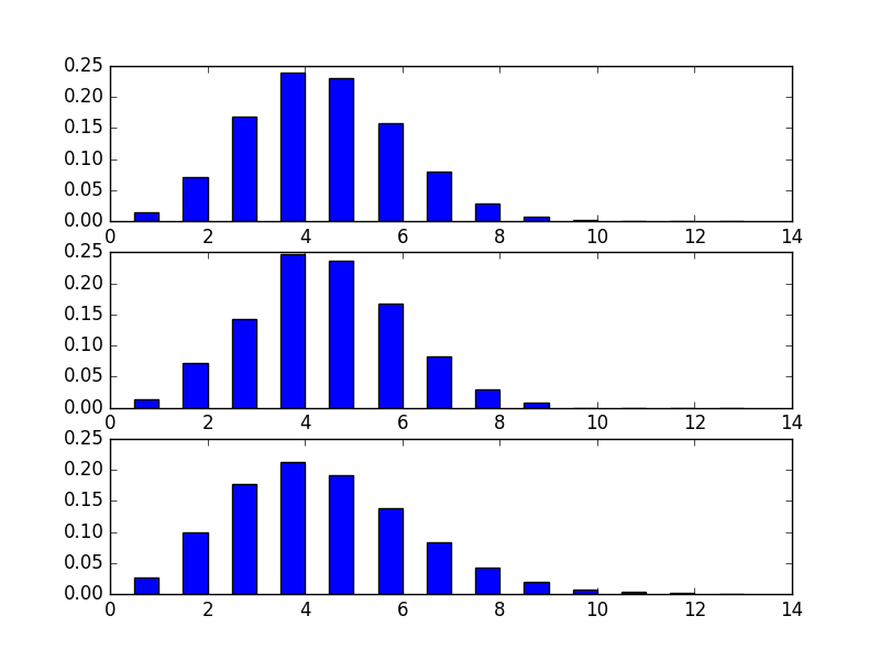
• In this week you have to plot three diagrams in a figure. The first diagram shows the binomial distribution with paramteres \((n,p)\). The second diagram shows the result of the simulation of this distribution. The third picture shows the first \(n+1\) columns of the diagram of the Poisson distribution with parameter \(\lambda=n\cdot p\) which approximates our binomial distribution.
• The output of this program will look like this (the scale and color is not an essential part of the figure):
  
• The inputs are \(n\), \(p\), \(k\), where \(n\) and \(p\) are the parameters of the binomial distribution, and \(k\) is the number of simulations. The program of Adrian Smith can be run by the next command:
  

  python 4AdrianSmith.py 12 0.3 1000

  or if using Python 3:

  python3 4AdrianSmith3.py 12 0.3 1000

  Using parameters in the command line you have to load the modul sys in the program. In this case the first parameter (in our example above the number 12) is contained by sys.argv[1] in character format, so you have to convert it (use the functions int or float). Test your program with different parameters like 20 0.05 1000, 40 0.02 1000 or 40 .5 1000.

• For the values of the binomial distribution you might need the binomial coefficients, what you can get from the math modul. The first diagram shows the binomial distribution.
• The simulation of this binomial distribution can be accomplished by executing $n$ times an event of probability $p$. The value of the random variable is $m$ if the event occurred $m$ times in the $n$ experiments. We repeat this $n$ experiment $k$ times so we get $k$ values of the random variable. The $m$-th column of the second diagram should be $i/k$ if the value of the random variable was $m$ exactly $i$ times from the $k$ values. (This part of the program can be written simply by loops using the random function of the random modul, or by the numpy.random.binomial function.)
• The third diagram shows the first $n+1$ values of a random variable $X$ of Poisson distribution with parameter $\lambda=np$, where \[ P(X=m)=\frac{\lambda^m}{m!}e^{-\lambda}, \quad m=0, 1, 2,\dots. \]
• For plotting the diagrams use the modul matplotlib. (I propose you to try firs this modul, it is very simply.) You can import this modul with
  

  import matplotlib.pyplot as plt

  after which

  plt.bar(list1, list2, columnwidth) 
  plt.show()
  

  draws a diagram where list1 is the list of the $x$-coordinates of the lower left corners of the columns, and list2 is the list of the height of the columns. The width of the columns is iven in the variable columnwidth. We want to present the three diagrams in a common figure, so before the first diagram use the function

  plt.subplot(311)

  where 311 means: the subfigures are in 3 lines and in 1 column, and this subfigure is the 1-st. Before next diagram use the number 312, and before the last one use 313. (The function plt.show() is enough to call at the end, but do not forget it.) 

• The aim of this exercise is to practice, simulate, approximate and better understand the binomial distribution.
• Programming goal is to learn the command line running of programs, plotting diagrams as subfigures.

5. Discrete random variables (deadline 2019-10-22 24:00, 5 points)

• Write a class called Drv (discrete random variable) for the interpretation of finite discrete random variables. The constructor of the class waits for two lists of the same length, the first contains the $x_k$ values of the random variable $X$, the second contains the probabilities $p_k=\mathbb{P}(X = x_k)$. Write the following methods:
  • __init__: constructor defines two attributes xk and pk for the two lists.
  • e: expected value of $X$.
  • is_nonneg: this method returns True if the random variable is non-negative, otherwise returns False.
  • reweighting: this method returns an instant of a random variable $Y$ from the original $X$ with the next "reweighting": \[\mathbb{P}(Y=x_k)=\frac{x_kp_k}{\mathbb{E}(X)},\] if $X$ is non-negative and has at least one nonzero value.
  • Binomial: A derived class from Drv for the binomial distribution. Parameters of this class are \(n\) and \(p\). Rewrite the code in this class for the e and for the is_nonneg methods.
  • Uniform: A derived class from Drv for the unifor distribution. The parameter of this class is \(n\), the list of values is \([1,2,\dots,n]\). Rewrite the methods mentioned above.
• During the writing and testing the code you may try the next interactive section:
  

  In [2]: y = Drv( [40, 33, 25, 50], [1/4]*4 )
  
  In [3]: y.xk
  Out[3]: [40, 33, 25, 50]
  
  In [4]: y.pk
  Out[4]: [0.25, 0.25, 0.25, 0.25]
  
  In [5]: y.is_nonneg()
  Out[5]: True
  
  In [6]: y.e()
  Out[6]: 37.0
  
  In [7]: x = y.reweighting()
  
  In [8]: x.xk
  Out[8]: [40, 33, 25, 50]
  
  In [9]: x.pk
  Out[9]: 
  [0.2702702702702703,
   0.22297297297297297,
   0.16891891891891891,
   0.33783783783783783]
  
  In [10]: x.e()
  Out[10]: 39.28378378378378
  
  In [11]: z = Binomial(5, .4)
  
  In [12]: z.xk
  Out[12]: [0, 1, 2, 3, 4, 5]
  
  In [13]: z.pk
  Out[13]: 
  [0.077759999999999982,
   0.25919999999999999,
   0.34560000000000002,
   0.23040000000000005,
   0.076800000000000021,
   0.010240000000000003]
  
  In [14]: z.e()
  Out[14]: 2.0
  
  In [15]: z = Uniform(3)
  
  In [16]: z.xk
  Out[16]: [1, 2, 3]
  
  In [17]: z.e()
  Out[17]: 2.0
  

• Please send the code of the class only and not the code of the usage of it showed above. For helping you we give a skeleton of the code for Python2 and Python3. You may read your code into an interactive section with the next commands. In Python2:
  

  from __future__ import division
  execfile("5YourName.py")
        

  In Python3:

  exec(open("5YourName3.py").read())
        

  After this, you may test your code with the function calls given above.

• Some help: please recall your knowledge about object oriented programming in Python, you may successfully use list comprehension, for the binomial coefficients you may import the comb function from scipy package with the command from scipy.special import comb .
• The purpose of this task is to write a system in object oriented programming style using heritage capable of handling discrete random variables.

6. Bertrand-paradox (deadline 2019-10-27 24:00, 5 points)

• The Bertrand paradox (in fact not a paradox) is an example of a seemingly simple probability variable can be achieved in a variety of ways if its definition is not clear enough. "The Bertrand paradox goes as follows: Consider an equilateral triangle inscribed in a circle. Suppose a chord of the circle is chosen at random. What is the probability that the chord is longer than a side of the triangle?" (from Wikipedia) Depending on the arguments, there are three possible valid answers: $1/2$, $2/3$ and $3/4$.
  1. The first assumption is to choose a random direction (by symmetry this can be any, so even the horizontal one) and the chord is selected from the perpendicular ones, randomly choosing a point on the horizontal diameter of the circle.
  2. The second assumption is to choose one point of the circumference of the circle and the other endpoint of the string is an other randomly chosen point.
  3. The third assumption is to choose a point from inside the circle (evenly distributed) and through it draw a string perpendicular to the line joining this point to center.
• All three assumptions and solutions (a bit differently formulated) with illustrative and enjoyable animations can be seen in a page of MIT. (Before reading this solution, you should think a little bit on it!)
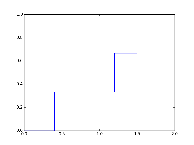
• Let the radius of the circle is 1, so its diameter is 2, and mark the string length in an experiment by $X$, i.e. $X$ is a probability variable with values between $0$ and $2$. The task will be to write a function bertrand (N), which simulates all three models $N$ times, records the lengths, and construct the three experimental cumulative distribution functions. The experimental cumulative distribution function at $x$ will say that how much is the relative frequency of the $\{X \lt x \}$ event. This is a step function. (The cumulative distribution function is defined by $F_X(x) = \mathbb P(X \lt x)$.) For example, if you make three experiments, and the string lengths are $ 1.5 $, $ 0.4 $ and $ 1.2 $, then the graph of the empirimental cumulative distribution function looks like this (the graph made by the step function of the matplotlib.pyplot library; do not worry about the vertical lines in the graph, and consider the function at these places continuous from the left):
  
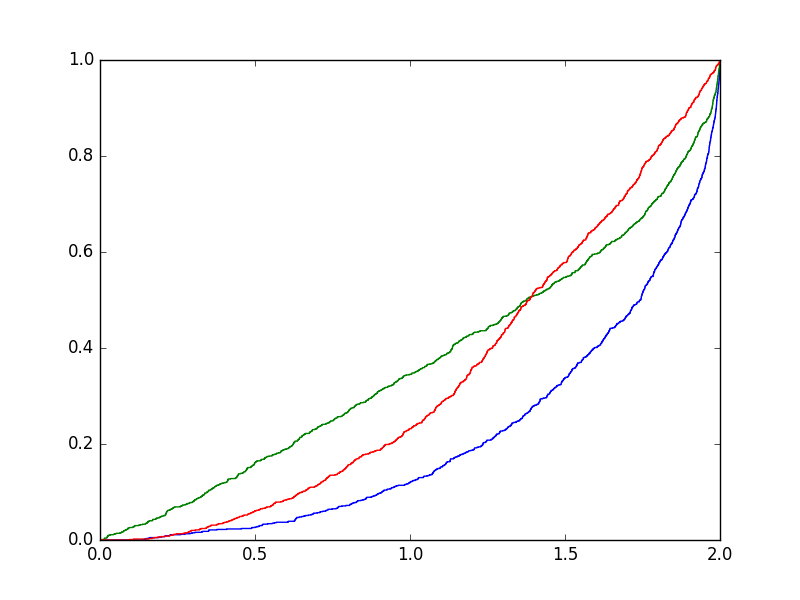
• The output of the task should be the graphs of the three experimental cumulative distribution functions in a single picture. The common domain is the interval $[0,2]$. Obviously all three functions are increasing, the value at $0$ is $0$, at $2$ is $1$, and the values at $\sqrt3 \approx1.732$ is approximately $1/2$, $2/3$, or $3/4$ depending on the model.
• A little help:
  • First model: choose a random number $r$ from the interval $[-1,1]$, and the calculate the length of the chord perpendicular to the horizontal line at $(r,0)$ (you may use the functions acos and sin from the modul math.
  • Second model: let the first point be $(1,0)$, and the second be a random point from the line of the circle, that is the point $(\cos\alpha,\sin\alpha)$, where $\alpha$ is a random number from the interval $[0,2\pi)$.
  • Third model: choose an arbitrary pont from the square $[-1,1]\times[-1,1]$ (that is choose two random numbers from the interval $[-1,1]$, and make a pair from them), and check if it is inside the circle. If not, choose an other one, and so on. The length of the chord can be calculated similarly to the first model.
  • Drawing the experimental cumulative distribution functions: after simulating $N$ experiments, sort the numbers with the sort() method. Write a $0$ at the beginning of the list and a $1$ at the end. This list gives the points on the horizontal axis. Above these points the step function "jumps." At each point the value of the function is increasing by $1/N$. If the length of the shortest cord is $r$, then the value of the function over $ [0, r] $ is $0$, so the list of function values is $y=[0,0,1/N,2/N,3/N,...,1]$. For drawing use matplotlib.pyplot.step(x,y) function where $x$ and $y$ are the two previously constructed lists. A possible result for $N=1000$ is shown in the following figure:
    
• After completing this program, do experiments with different values for $N$. Finally change the function step in the code to plot, and make your program runable from terminal. For example in the case $N=100$ execute the program with
  

  python 6AdrianSmith.py 100

  or in the case Python 3

  python3 6AdrianSmith3.py 100

• The aim of this task is to help understanding the continuous random variable, its cumulative distribution function and the approximation of it from experiments. There is no essential new topics in Python programming.

7. task: Simulate random variable with given cumulative distribution function (deadline: 2019-11-03  24:00, 3 points)

• The cumulative distribution function of a probability variable \(X\) on the interval \([0,2]\) is \(F_X(x) = x^2\), if \(x\in[0,0.5]\), and \(F_X(x)=(x+1)/3\), if \(x\in(0.5,2]\). Write a Python function that simulates a random variable with such a cumulative distribution function \(F_X\). Write a program that generates \(1000\) such random numbers and prints two numbers: their average and that how many of the \(1000\) numbers were equal to \(0.5\).
• The aim of the task is to understand the function of a random variable, for example to understand the random variable $F_X(X)$, and to use this to simulate a given random variable.

8. The party starts (deadline 2019-11-10  24:00, 5 points)

• Jack organizes a party for 10pm, inviting 10 friends. He found a special game that requires at least 8 players (besides him). Everyone is excited, so as soon as the 8th friend has arrived, he is starting the game. His friends arrive in a uniform distribution between 10 and 11pm (and no one arrives before 10, but everybody arrives until 11pm). Let $X$ denote the ratio of the starting time in the interval $[10,11]$ (ie. $X$ is a random variable with value between 0 and 1).
  1. Write a function simulating $X$!
  2. Consider the following two density functions: \begin{align*} f_a (x) = \frac{10!}{7! \cdot 2!}x^7 (1-x)^2, \quad 0\le x \le1,\\ f_b (x) = \frac{10!}{6! \cdot 3!}x^6 (1-x)^3, \quad 0\le x \le1. \end{align*} Simulate 5000 times the value of $X$, draw the histogram with 50 columns, draw the two density functions, and then decide which of them may be a density function of $X$.
  3. Using the previously generated 5000 data, substitute each simulated value of $X$ into both density functions and multiply the substituted value by a uniformly distributed random number from $[0,1]$ (independently generated from each other). Finally, these values as the function of the simulated values are drawn in a figure. For the two density functions we get two diagrams in this figure, they look like “cloud of points.” Decide which density function may belongs to $X$ based on these two diagrams. Give a short explanation of your answer.
• The output of the job is two figures. On the first there are two graphs of functions defined on \([0,1]\) and a histogram of 50 columns. The second figure consists of two subfigures, the top shows a cloud of points covering the area below the first density function, the lower shows a cloud of points covering the area below the second density function. In the e-mail, give a brief explanation of how and why could you read from the second figure which density function can be the real one of $X$.
• A little help:
  1. You may use the next code for drawing graphs (other good solutions are possible!):
     

     from __future__ import division  # if you use Python 2
     import numpy as np
     import matplotlib.pyplot as plt
     
     # t will be a list with elements 0, .02, .04,..., 1 
     step = 1/50
     t = np.arange(0, 1 + step, step)
     plt.plot(t, dfunc(t), color = "red")
     

     Here the first argument of the function plot is the list of the values of the domain, and the second argument contains the values of the function at these points, where dfunc have to be defined before.

  2. Drawing a histogram means drawing columns over intervals the height of which are proportional to the number of simulated values in the interval. There is a simple Python function to draw this histogram, where experiments is the list of the values of \(X\), bins is a list of values in the domain, normed means the total area of the columns:
     

     plt.hist(experiments, bins=t, normed=1)
     

  3. To draw points, you need to specify the style as the third argument of the function plt.plot, in this task it can be "r.", which means that the specified points will not be joined together, and the color of the points will be red (r = red).
• The aim of this exercise is to demonstrate the density function and simulate a given distribution (it is in this task the beta distribution, but it is not the part of the exercise to know or to understand this distribution!). Programming objectives are elementary programming and graphic skills.

9. Buffon's needle problem (deadline 2019-11-17 24:00, 3 points)

• Buffon's needle problem is a classic question, see for details in Wikipedia or in WolframMathWorld. We will generalize this question. Take a sufficiently large sheet of paper that has parallel lines with unit distances from each other. Drop a needle of length \(L\) randomly onto the paper. Let \(X\) be the number of lines touched by the needle. Write out the values of the frequency function of \(X\) based on the \(N\) experiments at 0, 1, 2, …, \(\lfloor L \rfloor + 1\).
• The command line input of the program is a positive integer number \(N\) and a positive real number \(L\), the output is a sequence of \(\lfloor L\rfloor+2\) integer numbers.
• We remark that if \(L=0.5\), then the relative frequency of the number of line-crossings is approximately \(1/\pi\).
• Simulation can be simplified because of symmetry reasons in several ways. For example, the angle between the needle and the lines can be considered a uniformly distributed variable on the interval \([0,\pi/2]\). Similarly, the distance of its center from the nearest line is uniformly distributed on \([0,0.5]\). One may calculate by supposing that the "left" end point of the needle is uniformly distributed on \([0,1]\), and so on.
• Those who love challenges may try to calculate the probabilities for a particular \(L\) (e.g. \(L = 2\) or \(L = 5\)) comparing the results with the experimental values. This isn't compulsory part of this exercise!

10. Convolution of dice with discrete U-shape distributions (deadline: 2019-11-24 24:00, 4 points)

• A biased dice gives the number $1$, $2$, $3$, $4$, $5$, $6$ appropriately with probability $0.35$, $0.10$, $0.05$, $0.05$, $0.15$, $0.30$. Throw some dice and calculate the sum of the numbers on them. Write a program which calculates (not simulates) the probabilities of these sums of one, two, three, four, ten, and twenty dice. After this, draw these six distribution functions. In the figure for the sum of the twenty dice, draw the density function of the normal distribution well approximating this sum with a different color.
• The aim of this exercise is the calculation of convolution, and visualization of the Central limit theorem.
• Help: The distribution of the convolution of $k$ dice can be determined from a set of $6^k$ elements, but such a program runs out of time. My advice: calculate the convolution of the distribution of $k$ dice recursively. First calculate the convolution of two dice from a diagonally summarized matrix. This distribution will have $11$ probabilities. For 3 dice, this distribution will be convoluted with the distribution of a dice. For this you may diagonally sum the elements of a $6\times11$ matrix. And so on.

11. Multivariate normal distribution (deadline: 2019-12-08 24:00, 5 points)

• This task illustrates an important relationship between the multidimensional and the one-dimensional normal distribution. The task is to produce 1000 points of 2-dimensional normal distribution with a given expected value and given covariance matrix and plot them on the plane. The figure has to be done in two ways! First, with the linear transformation of a random vector variable formed by two independent normal distributed random variable. For this you may use the function normal of the module numpy.random (and e.g. numpy.linalg). If \(\mathbf M\) denotes the transformation matrix, then the covariance matrix is \(\mathbf{M}\mathbf{M}^T\). Second, we generate random points by using the multivariate_normal function of the module numpy.random. One of the arguments of this function is the covariance matrix. Finally, draw the ellipse that contains most of the dots of the figure. The semi-axes of the ellipse be 6 times the singular values ​​of the covariance matrix (the singular value here coincides with the square root of the eigenvalue because the matrix is positve semidefinite). For simplicity, the expected value should be 0 and \((0,0)\).
• Run the program from command line. The arguments are the 4 elements of the transformation matrix. For example, the input line
  

  python 11AdrianSmith.py 2 5 3 0 

  means that the transformation matrix is \[ \begin{bmatrix} 2 & 5\\ 3 & 0 \end{bmatrix}, \] and the result of the program will be two figures like the following:
  

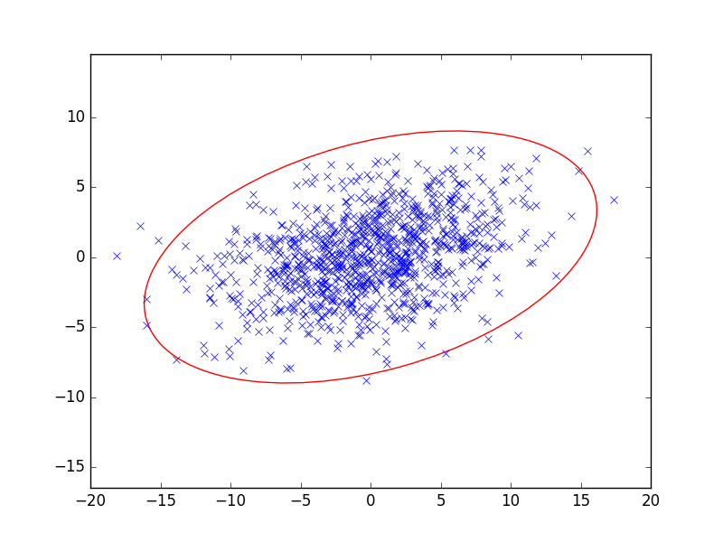
• Drawing the ellipses you need the lenght of the axes and the angle of the big axis with the horizontal $x$-axis. For this you may use the rad2deg and the arctan functions of the np module. A little help (not necessary to follow):
  

     from matplotlib.patches import Ellipse    # modul for drawing
  
     ax = plt.subplot(111, aspect='equal')     # subfigure
     ell = Ellipse(xy=(0,0),...                # fill in!
     ell.set_facecolor('none')                 # be empty
     ax.add_artist(ell)
     plt.plot(x, y, 'x')                       # these are the dots
     plt.axis('equal')
      

• The aim of the exercise is to demonstrate the relationship between the covariance matrix of 2-dimensional normal distribution and the linear transformation of a vector variable of independent normal distributions.

12. Zipf's law (deadline: 2019-12-08  24:00, 3 points)

The last task is about an interesting observation, which is called Zipf's law. Wikipedia writes: “Zipf's law was originally formulated in terms of quantitative linguistics, stating that given some corpus of natural language utterances, the frequency of any word is inversely proportional to its rank in the frequency table. Thus the most frequent word will occur approximately twice as often as the second most frequent word, three times as often as the third most frequent word, etc.: the rank-frequency distribution is an inverse relation.”

If this rule holds for a text, then the graph of the frequency function is a line in a coordinate system where both coordinate axes are logarithmic. The task will be to graphically check this rule for a natural text, that is, plot the frequencies in a loglog coordinate system. For testing some text samples can be found at http://sandbox.hlt.bme.hu/~gaebor/zipf/. This rule is perfectly implemented by the tokeletes.txt file in the text samples. There are smaller patterns with Hungarian text and larger with English text.

This time (as this is the last task) we give a big help as most of the program code is included, only the missing few lines has to be added. What to do can be figured out in the context and in the comments. The code runs under both Python2 and Python3.

from __future__ import print_function  # using print as a function

import matplotlib.pyplot as plt
import sys

filename = sys.argv[1]

def plot_zipf(filename):
    """
    Plot the frequencies of the words of a text
    and plot the rank-frequency function in a loglog
    coordinate system.
    """

    d = {}                                           # dictionary
    with open(filename, "r") as f:
        for line in f:
            for word in line.strip().split():        # split into words 
                word = word.strip(',.-_?! ').lower() # deleting punctuation
                if word != '':                  # count the nonempty words
                    ........                    # and write the frequences
                                                # into the dictionary d,
                                                # where the word is the KEY and
                                                # the frequency is the VALUE
                                     
    data = sorted(d.values(), reverse=True)          # a gyakorisagok
    plt.loglog(range(1, len(data)+1), data)          # kirajzolasa
    plt.show()                                       # loglog skalaval

    # convert the dictionary into a list of pairs, and sort by the
    # second element of the pairs and finally print the first 10 pairs
    print(sorted(d.items(), key=lambda x:x[1], reverse=True)[0:10])

def main():
    plot_zipf(filename)

if __name__ == "__main__":
    main()

This code runs a command-line executable form, but if someone writes and tests using jupyter, a line

%matplotlib inline

can be added as a second line in the code, but remove it from the file you are sending!

• The aim of the exercise is to get to know an empirical distribution and to choose the appropriate representation,
• getting to know the basics of processing natural language data.